How kernels are approximated in xGPR

An exact kernel machine measures the similarity of each training datapoint to every other training datapoint using a kernel function. This generally results in algorithms with at least O(N^2) scaling.

xGPR approximates the kernel matrix by representing each datapoint using a set of “random features”, a representation constructed such that the dot product between any two representations is approximately equivalent to the exact kernel measurement. This converts Gaussian process regression into ridge regression with O(N) scaling. xGPR uses an efficient fast Hadamard transform based procedure to do this, and incorporates a variety of “tricks” that dramatically speed up fitting for the resulting model, especially a randomized Nystrom preconditioner that reduces the number of epochs needed to fit by orders of magnitude.

The more random features you use, the more accurate the approximation and the closer to an exact kernel machine. The error decreases exponentially with the number of random features, so that if going from 1024 to 2048 random features improves model accuracy by a lot, going from 2048 to 4096 will improve it but not by as much, and then going from 4096 to 8192 will improve it but still less, and so on. The graph below illustrates how mean absolute error on held-out test sets for some (fairly random) UCI machine learning datasets decreases as the number of random features used for tuning hyperparameters or for fitting the model increases.

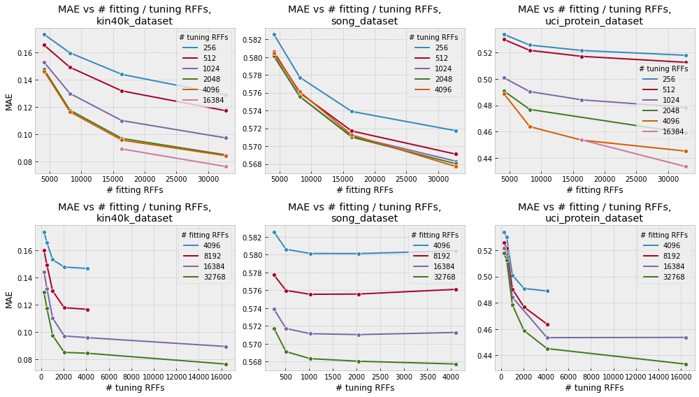
Notice that increasing the number of random features is nearly always beneficial, but with diminishing returns. This means that if our xGPR model is performing pretty well but we’d like it to perform a little better – just use more random features. If perforance is dramatically below what we need, by contrast, and increasing the number of RFFs isn’t helping very much, we know we need to switch to a different kernel, feature set or use another modeling technique instead of a GP.

How many random features do I need?

The hyperparameter settings that give good performance with a small number of random features are usually close to the ones that give good performance with a large number of random features. So, we like to use a small number of random features to pick a kernel and to figure out what region of hyperparameter space is likely best. By using a small number of random features (e.g. 1024 - 2048) we make these “screening” experiments fast. Once we’ve picked a kernel, we use a larger number of random features (e.g. 8192 - 16,384) to “fine tune” the hyperparameters and fit the model. See the quickstart tutorial and the examples on the main page for some illustrations.

As a general rule, the more high-dimensional the input data, the more RFFs you will likely need for an effective approximation. Thus, the RFF approximation (and xGPR in general) may not make sense if your data is very high-dimensional.

For regression models, xGPR also estimates the posterior predictive variance (i.e. the uncertainty) on new predictions. This generally only needs to be calculated very approximately. We recommend using 512 - 2048 random features for variance; this should be sufficient for an estimate in most cases. We often use 1024. The variance_rffs for variance calculation has to be < the num_rffs for predictions.